I recently saw this video on my YouTube landing page: some junior developer decided he would reimplement Shazam to keep himself busy and add something to his portfolio, since he can’t land a job. I decided to do it too, without looking at the video. After a few unsuccessful attempts, I gave up: I watched the video and read about the general algorithm ideas in a few different places. That guy’s implementation is extremely cool, and definitely more complete than mine, it is a fully-featured (almost) deployment-ready piece of software. But I’m not trying to make any money out of this, I just want to understand how Shazam works: let’s code Shazam in about 100 lines of Python.

The teasing: It will be able to extremely confidently recognize songs from such samples, among ~100 songs¹.

A physics crashcourse, a lie and a promise

Our goal is to design a fingerprinting algorithm for songs, so that even from an extremely partial and noisy sample from the song, we may recognize parts of its unique fingerprint and match it to the right song in our database. To design such a thing, we need to understand what is a .wav or .mp3 file in a computer, and this is actually closely related to what “sound” means in physics.

What’s a sound, really ?

Wikipedia states that:

In physics, sound is a vibration that propagates as an acoustic wave through a transmission medium such as a gas, liquid or solid. In human physiology and psychology, sound is the reception of such waves and their perception by the brain. Only acoustic waves that have frequencies lying between about 20 Hz and 20 kHz, the audio frequency range, elicit an auditory percept Sound waves above 20 kHz are known as ultrasound and are not audible to humans. Sound waves below 20 Hz are known as infrasound. Different animal species have varying hearing ranges, allowing some to even hear ultrasounds.

What matters in that paragraph is that our human ears hear sounds by sensing variations of the air pressure. In Audacity (a free software for editing audio files), when you open a file, you may visualize it like this:

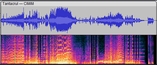
In the top part, a fairly familiar sight: the x-axis is time and the y-axis is the amplitude, i.e the pressure. As we just said, what really matters is the variation of that amplitude, so when we’re recording a sound numerically, we need to sample the air pressure very very often. Wikipedia states that we can hear sounds up to 20kHz, so we need atleast 20 000 samples per second ! Actually, to avoid aliasing it is better to have atleast twice that, i.e 40kHz. In a computer, if we ignore compression to save memory, a sound will be represented as a header with some metadata (notably the duration, the sample rate and the number of channels) and then a big list of all these samples. This is exactly how the .wav file format is designed.

Back to that image: in the bottom part, we see something completely different. The x-axis is still time, and the color is the intensity of the sound at a given time, but then what’s the y-axis ? The answer is frequency, in this case it seems to be varying between 0 and 12kHz, with most signal being below 2.6kHz. As I am more a mathematician than a physicist, I understand this through the following theorem from Fourier analysis:

For $f: \mathbb{R} \to \mathbb{R}$ sufficiently smooth (for instance, $\mathcal{C}^1$ is enough) and $1$-periodic, there exists a unique sequence $(a_n)_{n \in \mathbb{Z}}$ such that

$$f(x) = \sum_{n \in \mathbb{Z}} a_n e^{2 i \pi n x}$$

Moreover the coefficients $a_n$, called the frequencies composing $f$, can be retrieved through the formula

$$a_n = \int_0^1 f(x) e^{-2i \pi nx} \mathrm{d}x$$

The second part of that statement is easy to deduce from the first, by swapping both integrals and using the identity $\int_0^1 e^{2 i \pi n x} = 0$ whenever $n \neq 0$. The first part requires some work and I we will not go down this rabbit hole. Going back to the physics, if we think of $f$ as representing a sound (that is the air pressure as a function of the time), we see that any (periodic, it will matter later) sound can be decomposed as a sum of pure trigonometric waves. Pure sin/cosine soundwaves are called pure tones in music, and they sound kind of like when you hit a single note on a piano.

The infamous FFT

Leaving the physicist realm, we go back to our computers: given an audio file, we need a way to go from the amplitude representation to the frequency representation. The above theorem (up to discretization, i.e replacing integrals by sums over the points of the sampling grid), this amounts to computing enough fourier transforms, that is the above integrals ², which is about 2 * SAMPLE_RATE ^2 * DURATION_IN_SECONDS operations. Even at the extremely low SAMPLE_RATE = 12_000 for a 3 min audio, we would need 25 920 000 000 operations. Luckily for us, there is a clever algorithm designed in a divide-and-conquer fashion that speeds up this process significantly and runs in quasi-linear time: the Fast Fourier Transform (FFT). For a fairly clear explanation of the algorithm, see this wikipedia page.

Spectrograms

I actually put something under the rug earlier, when I talked about that frequency sound representation (which is called a spectrogram btw). We have a tool (the Fourier transform) to extract frequencies from a sound, but how do we extract frequencies for a sound.. at a given time $t_0$. It turns out we cannot do that, so we do the next best thing: we pick a very small window $[t_0 - \varepsilon, t_0 + \varepsilon]$ and use the Fourier Transform to extract the frequencies of that new sound. Sadly, Fourier transform is designed to work on periodic signal and there is no reason to believe that sound will be periodic. The discontinuities at the edges introduce aliasing defects, and to avoid that we use a smoothing window function $\omega(t)$ that is supported on $[t_0 - \varepsilon, t_0 + \varepsilon]$ and zero elsewhere, and we take the Fourier transform of the sound multiplied by this window function over a larger time frame. This avoids aliasing almost completely, at the expense of introducing parasitic frequencies that come from the window function.

Listing the dependencies

In essence, the algorithm is fairly easy to map into pure, clean and simple Python, but it will never be fast enough for comfortable use. I wanted to be able to quickly iterate over changes and waiting 20 secondes every time I need the frequency representation of my 3 minute audio was not an option, so I used the librosa library in Python. Similarly, audio files I/O is also handled by librosa, even though .wav is fairly simple and I could have just parsed it by hand. For speed, comfort and many other very good reasons, I also use numpy.

That’s it, we are set up, no more new specific theory, no more dependencies. The rest is really about 100 line of codes of pure Python, and a working reasonable proof-of-concept Shazam clone that works reasonably fast with very good noise and distortion resistance (see below for some tests). No magic theorem or unknown data structure, that’s a promise !

The strategy

Here’s a rough outline of what we will do for each audio we want to be able to recognize:

• Preprocess our audio: resample it to a fixed sample rate, average across channels to transform stereo signals to mono
• Apply the procedure explained above to get a spectrogram out of our signal
• Split the spectrogram into a few frequency bands (pretty much given by octaves), to avoid dominance in magnitude by the low bass that are often amplified in musical post-processing³
• For each of these bands, store the local magnitude peaks in a big database, that is store triples (peak_frequency, sample_index, music_name). We’ll make the meaning of “local magnitude peak” more precise below, but you can think of it as “the fundamental note played at a given moment in a given octave”

Then, when we’re querying the database with a given noisy recording, we apply the same steps but instead of storing the peaks in the database, we collect all the matching peak_frequencies in the database and then we compare the sample indexes of the matches against the sample indexes of the noisy recording. If there is enough match for a given song and they are coherent in timing, then we found a very likely match.

The data

I used the yt-dlp library/command-line tool to download a few famous musical .wav files from YouTube and put them in a audios/ folder at the root of the project. The list is composed of about 100 very famous songs ChatGPT put together + 3 randoms songs I added in there (can you find them ?). Note that I downloaded everything as .wav files because I wanted everything to be as simple as possible, but in real life you would definitely use .mp3 files.

import yt_dlp
from pathlib import Path

def download_batch_as_wav(queries, output_dir):
    output_dir = Path(output_dir)
    output_dir.mkdir(parents=True, exist_ok=True)

    base_opts = {
        "format": "bestaudio/best",
        "noplaylist": True,
        "default_search": "ytsearch1",
        "postprocessors": [
            {
                "key": "FFmpegExtractAudio",
                "preferredcodec": "wav",
            }
        ],
        "postprocessor_args": ["-ar", "12000"],
        "quiet": False,
    }

    for query in queries:
        filename = query.lower().replace(' - ', '__').replace(' ', '_')

        ydl_opts = base_opts | {
            "outtmpl": str(output_dir / f"{filename}.%(ext)s")
        }

        with yt_dlp.YoutubeDL(ydl_opts) as ydl:
            print(f"Downloading: {query}")
            ydl.download([query])

songs = [
        "Bohemian Rhapsody - Queen",
        "Imagine - John Lennon",
        "Billie Jean - Michael Jackson",
        "Hey Jude - The Beatles",
        "Like a Rolling Stone - Bob Dylan",
        "Smells Like Teen Spirit - Nirvana",
        "Hotel California - Eagles",
        "Sweet Child O' Mine - Guns N' Roses",
        "Stairway to Heaven - Led Zeppelin",
        "I Will Always Love You - Whitney Houston",
        "Thriller - Michael Jackson",
        "Rolling in the Deep - Adele",
        "Someone Like You - Adele",
        "Purple Rain - Prince",
        "Let It Be - The Beatles",
        "Yesterday - The Beatles",
        "Hallelujah - Leonard Cohen",
        "Uptown Funk - Mark Ronson ft. Bruno Mars",
        "Shape of You - Ed Sheeran",
        "Blinding Lights - The Weeknd",
        "Wonderwall - Oasis",
        "Lose Yourself - Eminem",
        "What a Wonderful World - Louis Armstrong",
        "Comfortably Numb - Pink Floyd",
        "Born to Run - Bruce Springsteen",
        "Take On Me - a-ha",
        "Every Breath You Take - The Police",
        "Africa - Toto",
        "Justin Timberlake - Can't Stop The Feeling",
        "Livin' on a Prayer - Bon Jovi",
        "I Want It That Way - Backstreet Boys",
        "Single Ladies - Beyoncé",
        "Crazy in Love - Beyoncé",
        "No Woman No Cry - Bob Marley",
        "Redemption Song - Bob Marley",
        "Superstition - Stevie Wonder",
        "Isn't She Lovely - Stevie Wonder",
        "Karma Police - Radiohead",
        "Creep - Radiohead",
        "Firework - Katy Perry",
        "Bad Romance - Lady Gaga",
        "Poker Face - Lady Gaga",
        "Take Me to Church - Hozier",
        "Thinking Out Loud - Ed Sheeran",
        "All of Me - John Legend",
        "Clocks - Coldplay",
        "Viva La Vida - Coldplay",
        "Fix You - Coldplay",
        "Paramore - Misery Business",
        "My Heart Will Go On - Celine Dion",
        "Toxic - Britney Spears",
        "Baby One More Time - Britney Spears",
        "Smooth - Santana ft. Rob Thomas",
        "With or Without You - U2",
        "Beautiful Day - U2",
        "September - Earth, Wind & Fire",
        "Stayin' Alive - Bee Gees",
        "Dancing Queen - ABBA",
        "Mamma Mia - ABBA",
        "Take Me Home, Country Roads - John Denver",
        "American Pie - Don McLean",
        "Dream On - Aerosmith",
        "Back in Black - AC/DC",
        "Thunderstruck - AC/DC",
        "Eye of the Tiger - Survivor",
        "Nothing Else Matters - Metallica",
        "Enter Sandman - Metallica",
        "Radioactive - Imagine Dragons",
        "Believer - Imagine Dragons",
        "Despacito - Luis Fonsi ft. Daddy Yankee",
        "Old Town Road - Lil Nas X",
        "Bad Guy - Billie Eilish",
        "Rolling Stone - The Weeknd",
        "MPH - Cadence", 
        "God's Plan - Drake",
        "One Dance - Drake",
        "Lose Yourself to Dance - Daft Punk",
        "Get Lucky - Daft Punk",
        "Call Me Maybe - Carly Rae Jepsen",
        "Fireflies - Owl City",
        "Shake It Off - Taylor Swift",
        "Blank Space - Taylor Swift",
        "We Will Rock You - Queen",
        "We Are the Champions - Queen",
        "Sweet Caroline - Neil Diamond",
        "Take Me Out - Franz Ferdinand",
        "Mr. Brightside - The Killers",
        "Seven Nation Army - The White Stripes",
        "Paint It Black - The Rolling Stones",
        "Gimme Shelter - The Rolling Stones"
]

For benchmarking, I also recorded with my phone in noisy environments/squashed together through scripting and audacity diverses kind of noisy recordings, either by adding a noisy cafe environment, adding gaussian noise or recording over with my phone and talking over it. All of these got recognized by the algorithm, needing at most 20 seconds of recording for the most noisy environments (approx. signal to noise ratio equal to 1).

The code

Building the database

Let’s start with a rough pseudo-code:

def build_database(audios: list[(str, str)]):
    database = empty_database()
    for (audio_path, tag) in audios:
        audio = load_audio(audio_path)
        spectrogram = build_spectrogram(audio)
        bands = get_bands(spectrogram)
        for band in bands:
            (peaks, magnitudes, sample_indexes) = get_peaks(band)
            for (peak, magnitude, sample_idx) in zip(peaks, magnitudes, sample_indexes):
                database[peak].append((tag, sample_idx))
    return database

Let’s implement that line by line. For the database we use a collections.defaultdict, which is simply a hashmap with a default value in case the key does not exist. In this case, the default value is an empty list.

from collections import defaultdict

def build_database(audios):
    database = defaultdict(list)

We load the audio with

audio, _ = librosa.load(audio_path, sr=SAMPLE_RATE, mono=True, dtype=np.float32)

There’s actually lot happening here, so let’s go through the parameters one by one:

• We load the audio by giving its path to librosa
• We force librosa to resample⁴ it to the given SAMPLE_RATE constant. The reason we resample is 1) we want all our audios to have the same frequency bands and 2) to reduce the computational load 3) the main melodic frequencies lie below 4kHz, so we don’t need more than twice the samples per seconds to hear them without aliasing. YouTube audios have a default sample rate of 44kHz, definitely too much for signal analysis. We set SAMPLE_RATE = 8_000. There will be a lot of tunable constants like these along the way so we’ll add them one after another at the beginning of the file.
• We ask it to give a mono (i.e 1-dimensional, as opposed to hearing different things in both ears when you wear headphones for instance). This is simply done by averaging over all the channels.
• Finally, we ask for our signal to be read as 32bit floating points numbers.

The second argument we ignore with _ is the sample rate, which is useful if you let the sr parameter unspecified and work with files coming with distinct sample rates: not our case.

Next, we need the spectrogram of our signal. As explained above, we need to take the fft of our signal times a smoothing function supported on a small subset. We could define such a function like this

def build_spectrogram(audio, window_size, hop_length, smoothing_window):
    """
    smoothing_window is a window_size-sized array
    """
    frames = 1 + (len(audio) - window_size) // hop_length 

    spectrogram = np.zeros((frames, 1 + window_size // 2), dtype=np.complex)
    for i in range(0, len(audio), hop_length)
        if i + window_size >= len(audio):
            break
        spectrogram[k, :] = np.fft.rfft(audio[i:i+window_size] * smoothing_window)
    return np.abs(spectrogram)

We make use of numpy’s real fft function⁵. Note that we take the absolute value since we are only really interested in the magnitude of the signal, not the phase.

The nice thing about librosa is that it already provides a function that builds a spectrogram out of our audio, so that we don’t have to handle the sliding window ourselves (and make it a speed bottleneck). It is called stft for Short-Time Fourier Transform

spectrogram = np.abs(librosa.stft(audio, n_fft=WINDOW_SIZE, hop_length=HOP_LENGTH, window="hamming"))

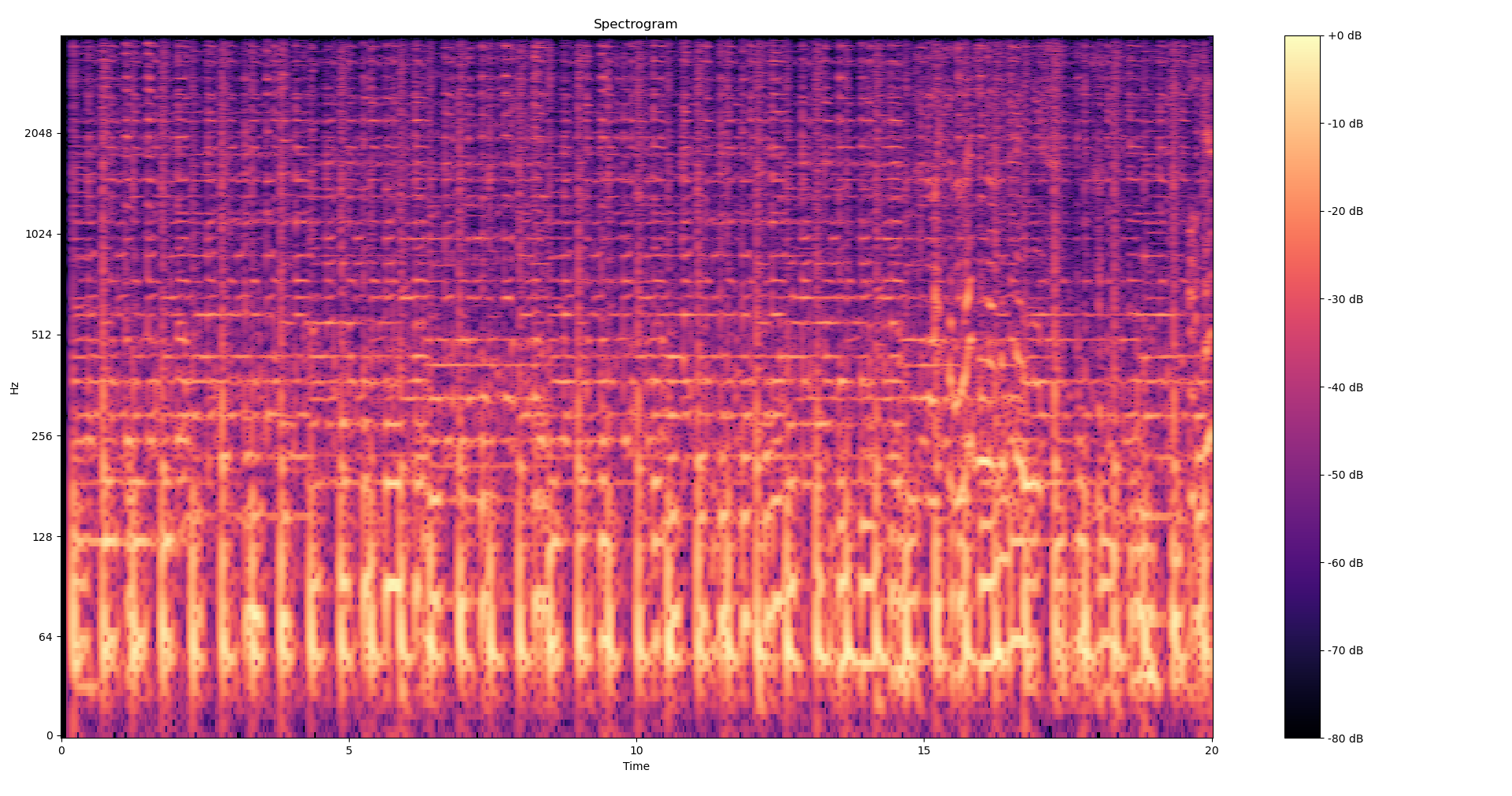
For the constants, we set at the beginning of the file WINDOW_SIZE = 2048, HOP_LENGTH = 256 which are approximately equal to 250ms and 25ms, given a sampling_rate of 8000. The window="hamming" parameter tells librosa to use a Hamming smoothing window function. Why this function and not another one ? It seems to be the one that better preserves peak frequencies. I checked that by drawing the spectrograms of a few sums of sinusoids with matplotlib.

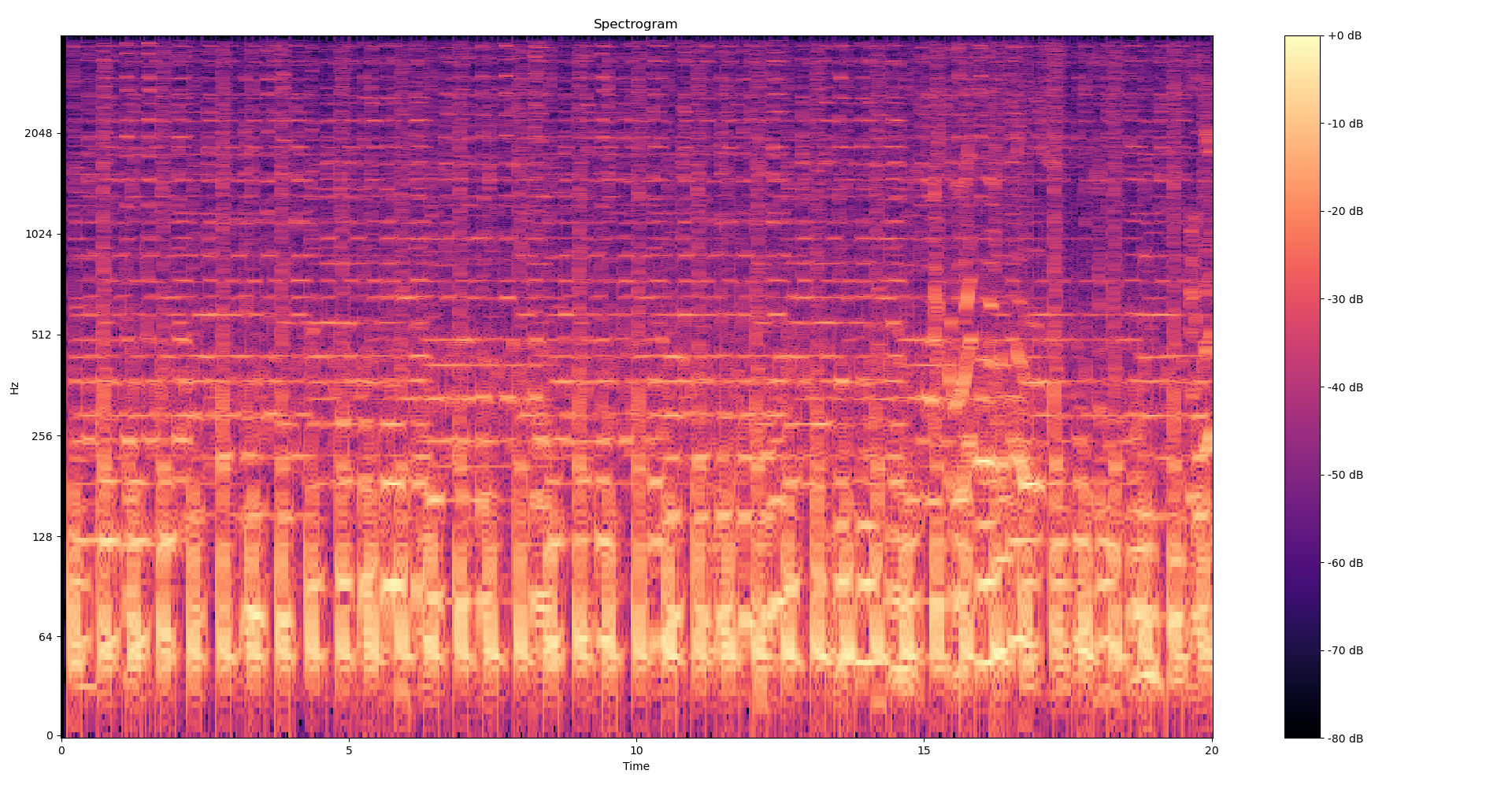
To get a better feel as to what we’re doing here, Here is the spectrogram of the 20 first seconds of Get Lucky from the Daft Punk, first built with a hamming window and then without any smoothing window (i.e a rectangular window). We can clearly see the rough cut-offs created by the aliasing in the second picture.

Now we want to split our spectrogram into frequency bands. Frequencies below 80Hz can safely be dropped since they’ll often contain more noise than signal, and anything above 1300Hz is already extremely high. We thus define the following bands: 80-160Hz, 160-320Hz, 320-640Hz, 640-1280Hz, 1280-4000Hz. We’ll need to index our spectrogram, i.e map these frequencies to actual spectrogram indexes, and so we define

STFT_RESOLUTION = SAMPLE_RATE / WINDOW_SIZE

BAND_THRESHOLDS = [80, 160, 320, 640, 1280, SAMPLE_RATE // 2]
BAND_INDEXES = [
    (
        round(BAND_THRESHOLDS[i] / STFT_RESOLUTION),
        round(BAND_THRESHOLDS[i + 1] / STFT_RESOLUTION),
    )
    for i in range(len(BAND_THRESHOLDS)-1)
]

In the build_database function we define

    bands = [spectrogram[start:end, :] for (start, end) in BAND_INDEXES]

Now to compute the peaks, we need to define what’s a peak: a peak in a band is a frequency whose magnitude is maximal among a rectangular neighborhood of size FREQ_NGHBR x TIME_NGHBR. We think of each band as an image and apply a maximum filter to it, then compare it with the original image to get a boolean array of peak locations. We remove the peaks whose intensity lie below the bottom INTENSITY_THRESHOLD% of points in the band, as they are likely to be noise. Finally, we reindex the frequency indexes of the peaks to go from band index to global (spectrogram) index and store all of that in a.. list of tuple of lists.

from scipy.ndimage import maximum_filter

peaks = []
for band_idx, band in enumerate(bands): 
    local_maximums = band == maximum_filter(band, size=(FREQ_NGHBR, TIME_NGHBR))
    thresh = np.percentile(band, INTENSITY_THRESHOLD)
    strong = band >= thresh

    (band_freq_indexes, sample_indexes) = (local_maximums & strong).nonzero()
    global_freq_indexes = band_freq_indexes + BAND_INDEXES[band_idx][0] # 
    peaks.append(global_freq_indexes, sample_indexes)

We also set the constants

INTENSITY_THRESHOLD = 95
FREQ_NGHBR = 30
TIME_NGHBR = 15

I have no strong reason for these numerical choices, they worked correctly but there’s probably a lot of fine-tuning to be done on these. Finally, we iterate over this list of list and append each peak in the database dictionary, with the additional information of the timing of the ping (the sample_index) and the tag of the song, and we return the database at the end. Here is the final code for the database

def bands_peaks(spec):
    bands = [spec[start:end, :] for (start, end) in BAND_INDEXES]
    peaks = []
    for band_idx, band in enumerate(bands): 
        local_maximums = band == maximum_filter(band, size=(FREQ_NGHBR, TIME_NGHBR))
        thresh = np.percentile(band, 95)
        strong = band >= thresh
        (band_freq_indexes, sample_indexes) = (local_maximums & strong).nonzero()
        global_freq_indexes = band_freq_indexes + BAND_INDEXES[band_idx][0]
        peaks.append((global_freq_indexes, sample_indexes))
    return peaks

def build_database(audios, path="database.json"):
    try:
        with open(path, "r") as db:
            database = json.load(db)
            # Integers keys got converted to strings during json serialization
            return defaultdict(list, {int(k):v for k,v in database.items()})
    except FileNotFoundError:
        pass

    database = defaultdict(list)
    for (audio_path, tag) in audios:
        print(f"Adding {tag} to database")
        audio, _ = librosa.load(audio_path, sr=SAMPLE_RATE, mono=True, dtype=np.float32)
        spectrogram = np.abs(librosa.stft(audio, n_fft=WINDOW_SIZE, hop_length=HOP_LENGTH, window="hamming"))
        peaks = bands_peaks(spectrogram)

        for freq_indexes, sample_indexes in peaks:
            for freq, sample in zip(freq_indexes, sample_indexes):
                database[int(freq)].append((int(sample), tag))
    
    with open(path, 'w') as file:
        json.dump(database, file, indent=2)
    
    return database

I extracted the bands_peaks logic in another function since we’ll reuse it in the next section. I also added some basic saving/loading of the database in a JSON file, since recomputing the database everytime is annoying.

Matching a recording

To match a recording to the database we built, we first compute its spectrogram and extract the band peaks. Then, for each of the recording’s peak, we compare the matching frequencies in the database and we compute the offset (time/sample_index difference) between the database peak and the recording peak. If a given song has enough matching offsets, we found a likely match !

from collections import Counter

# Some testing showed allow for a little margin for the scoring helped getting more robust scores, 
# since on noisy data the magnitude peaks may happen a few m.s before/after the peak on the original audio

def score_offsets(offsets, window=2):    
    offsets_counts = Counter()

    for t_audio, t_query in offsets:
        offset = t_audio - t_query
        for i in range(max(0, offset - window), offset + window + 1):
            offsets_counts[i] += 1
    _dominant_offset, count = offsets_counts.most_common(1)[0]
    
    return count

def match_recording(database, recording_path):
        recording, _ = librosa.load(recording_path, sr=SAMPLE_RATE, mono=True, dtype=np.float32)
        spectrogram = np.abs(librosa.stft(recording, n_fft=WINDOW_SIZE, hop_length=HOP_LENGTH, window="hamming"))
        rec_peaks = bands_peaks(spectrogram)

        offsets = defaultdict(list)
        for rec_freq_peaks, rec_sample_peaks in rec_peaks:
            for rec_freq_idx, rec_sample_idx in zip(rec_freq_peaks, rec_sample_peaks):
                for db_sample_idx, tag in database[rec_freq_idx]:
                    offsets[tag].append((db_sample_idx, rec_sample_idx))
        scores = []
        for tag, offsets_array in offsets.items():
            score = score_offsets(offsets_array)
            scores.append((tag,score))
        
        return sorted(scores, key= lambda x: x [1], reverse=True)

Final results, benchmarks and last words

The full code is available here, on GitHub, without the songs since they’re obviously too large, but the download script is available for the songs. I also included the 2 samples I showed earlier, but test it with your own samples also! Including imports, constants definition and the pretty printing of the results, we are at 107 lines of code, with only about 50 lines of logic: I kept up on that promise!

Here are the results with the 2 samples I shared at the beginning of the post. I feel like that’s pretty solid, given the amount of noise.

Querying file samples/noisy_sample2__britney_spears__toxic.wav
Top 2 scores
Song toxic__britney_spears scored 44
Song every_breath_you_take__the_police scored 19
-----------------------------------------------------
Querying file samples/noisy_cafe__beyonce__crazy_in_love.wav
Top 2 scores
Song crazy_in_love__beyoncé scored 558
Song lose_yourself__eminem scored 31
-----------------------------------------------------

Many improvements are possible:

• All of the matching is pretty fast but could be made significantly faster by using pairs of temporally close peaks instead of singles peaks as keys for the database. That would drastically reduce the number of useless matches.
• All these arbitrary defined constants could be tuned to better match the reality of noisy musics we hear outside
• We could make things faster by first trying to use only the first 5 seconds of the recording, then the 10 first seconds etc, as the real Shazam does. Often the audio will be clear enough that 5 seconds will. etc.

Comments

Sorry, I’m too lazy to load a proper comment system plugin: see the associated github issue.